Cubic Spline Interpolation

by Ryan Anderson and Heidi Scarff

The most common piecewise polynomial approximation uses cubic polynomials between each successive

pair of nodes and is called cubic spline interpolation. The following will show how to use two kinds of cubic spline interpolations, natural cubic spline and clamped cubic spline. These methods are easier than Hermite interpolation because they do not require us to know the derivatives, except at the endpoints of the intervals being approximated. There is sufficient flexibility in this procedure to ensure that the interpolant has a continuous first and second derivative on the interval.

Definition of a Cubic Spline Interpolation (3.10)

Given a function f defined on [a,b] and a set of nodes a = x0 < x1 << xn = b, a cubic spline interpolant S for f is a function that satisfies the following conditions:

a. S(x) is a cubic polynomial. It is denoted Sj (x) on the interval [xj , xj+1] for each j = 0,1,n-1; i.e. S0(x) is on the subinterval [x0 , x1]

a. S(xj) = f(xj) for each j = 0,1,2,,n; Note: we cannot assume that the derivatives of the interpolant agree with those of the function, even at the nodes. f'(x)S'(x)

b. Sj+1(xj+1) = Sj(xj+1) for each j = 0,1,2,,n-2;

c. S'j+1(xj+1) = S'j(xj+1) for each j = 0,1,2,,n-2;

d. S''j+1(xj+1) = S''j(xj+1) for each j = 0,1,2,,n-2;

e. One of the following boundary conditions is true:

i) S''(x0) = S''(xn) = 0 free or natural boundary

ii) S'(x0) = f'(x0) and S'(xn) = f'(xn) clamped boundary

When the free boundary conditions occur, the spline is called a natural spline. The clamped boundary conditions lead to more accurate approximations because they include more information about the function. However, it is necessary to have either the values of the derivatives at each endpoint or a close approximation.

Solving for coefficients

To construct the cubic spline interpolant for a given function f, we need to solve for the coefficients a,b,c, and d. To do this, the conditions in the definition are applied to the cubic polynomials of the form

Sj(x) = aj+ bj(x - xj) + cj(x - xj)2 + dj(x - xj)3

for each j = 0,1,,n-1.

From here we can easily see that

Sj(xj) = aj = f(xj).

Now if we apply condition ( c ) of the definition above

(1) Sj+1(xj+1) = aj+1 which implies

(2) aj+1 = Sj+1(xj+1) = Sj(xj+1) = aj + bj(xj+1 - xj)

+ cj(xj+1 - xj)2 + dj(xj+1 - xj)3

for each j = 0,1,,n-2.

To make things a little easier, let

(3) hj = xj+1 - xj

for each j = 0,1,,n-1.

Now, define an = f(xn). Then

(4) aj+1 = aj + bjhj + cjh2j + djh3j

holds for each j = 0,1,,n-1.

Similarly, we can define bn = S'(xn).

(5) S'j (x) = bj +2cj (x - xj )+ 3dj (x - xj )2

Which implies that S'j(xj) = bj for each j = 0,1,,n-1.

Applying condition (d) gives

(6) bj+1 = bj + 2cj hj + 3dj h2 j

for each j = 0,1,,n-1.

Now define cn = (S''(xn)/2).

Applying condition (e) gives

(7) cj+1 = cj + 3dj hj

for each j = 0,1,,n-1.

Solving for dj in (7) and the substituting this value into (5) and (6) gives the following equations.

(1) aj+1 = aj + bj hj +(1/3)h2 j( 2j + cj+1)

and

(1) bj+1 = bj + hj (cj+cj+1)

for each j = 0,1,,n-1.

Next, solve equation (8) first for bj.

(1) bj=(1/ hj)(aj+1 - aj) -(1/3) hj(2cj + cj+1)

Now, reduce the index of (10) to bj-1 and the equation becomes:

(1) bj-1 = (1/hj-1)(aj - aj-1) -(1/3) hj-1(2cj-1 + cj)

Substitute these values into (9), with a reduced index of one. This produces the following linear systems of equations:

(1) h_j-1c_j-1 +2(h_j-1-h_j)c_j + h_jc_j+1 = (1/3)h_j(a_j+1-a_j)-(3/h_j-1)(a_j-a_j-1),

for each j = 1,2,,n-1.

Theorem 3.11 (p.147)

If f is defined at a = x0< x1<< xn = b, then f has a unique natural spline interpolation on the nodes x0, x1, , xn. In other words, it has a spline the satisfies the boundary conditions S''(a) = 0 and S''(b)=0.

Natural Cubic Spline (Algorithm 3.4 p.148)

To construct the cubic spline interpolant S for the function f, defined at the numbers x0< x1<< xn, satisfying S''(x0) = S''(xn) = 0.

INPUT n; x0 , x1 , , xn;a0 = f(x0), a1= f(x1), , an = f(xn).

OUTPUT ai , bi , ci , di for i = 0,1,,n-1. (Note: S(x) = Si(x) = ai+ bi(x - xi) + ci(x - xi)2 +

di(x - xi)3 for xi<= x<= xi+1.)

Step 1 For i = 0,1,,n-1 set

hi = xi+1 - xi.

Step 2 For i = 1,2,,n-1 set

yi = (3/hi )(ai+1 - ai) - (3/hi-1)(ai -ai-1).

(Steps 3-5 and part of Step 6 solve a tridiagonal linear system using the method described in Algorithm 6.7)

Step 3 Set l0 = 1;

u0 = 0;

z0 = 0;

Step 4 For i = 1,2,,n-1 set

li = 2(xi+1 - xi-1) - hi-1ui-1;

ui = hi/li

zi = (yi - hi-1 zi-1)/li.

Step 5 Set ln = 1;

zn = 0;

cn = 0;

Step 6 For i = n-1,n-2,,0 set

ci = zi - ui ci+1;

bi = (ai+1 - ai)/hi - hi(ci+1 +2 ci)/3;

di = (ci+1 - ci)/(3hi);

Step 7 OUTPUT (ai , bi , ci , di for i = 0,1,,n-1)

STOP.

Theorem 3.12 (p148)

If f is defined at a = x₀<x₁<... < x_n = b and differentiable at a and b, then f has a unique clamped spline interpolant on the nodes x₀, x₁,...,x_n, that is a spline interpolant athat satisfies the boundary conditions S'(a)=f'(a) and S'(b)=f'(b).

Clamped Cubic Spline Algorithm (3.5)

Input:

n,

x₀...x_n

a_i=f(x_i) , 0<=i<=n

FPO = f'(x_o)

FPN = f'(x_n)

Output:

a_j,b_j,c_j,d_j for j=0,1...n-1

Step 1 for i=0,1,...,n-1 set hi=xi+1 - xi

Step 2 Set ₀ = 3(a₁-a₀)/h₀ - 3*FPO

_n=3*FPN-3(a_n-a_n-1)/h_n-1

Step 3 For i=1,2,...,n-1

set _I = 3/h_i (a_i+1-a_i)-3/h_i-1(a_i-a_i-1)

Step 4 Set l₀ = 2h₀

µ₀ = 0.5

z₀ = ₀/l₀

Step 5 For i=1,2,...,n-1

set li = 2(xi+1 - xi-1) - hi-1µi-1

µ_i - h_i/l_i

z_i = (_i-h_i-1z_i-1)/l_i

Step 6 Set l_n = h_n-1(2-µ_n-1)

z_n = (_n-h_n-1z_n-1)/l_n

c_n=z_n

Step 7 For j=n-1,n-2,...,0

set c_j=z_j-µ_jc_j+1

b_j=(a_j+1-a_j)/h_j - h_j(c_j+1+2c_j)/3

d_j=(c_j+1-c_j)/(3h_j)

Step 8 Output (a_j,b_j,c_j,d_j, for j=0,1,...,n-1)

Stop.

Algorithm 3.4 - Output

This is the output from algorithm 3.4, solving problem 11 from page 155:

The total number of intervals = 4

Enter the numbers x

0.0

0.25

0.5

0.75

1.00

Now the values of f(x):

1.0

0.707107

0.0

-0.707107

-1.0

i x[i] a[i] b[i] c[i] d[i]

0 0 1 -0.757358 0 -6.62742

1 0.25 0.707107 -2 -4.97057 6.62742

2 0.5 0 -3.24264 -1.0842e-19 6.62742

3 0.75 -0.707107 -2 4.97057 -6.62742

This agrees substantially with the answer on page 746

Implementation:

#include <iostream.h>

#include <math.h>

void main()

{ int i,n;

long double *x,*h,*y,*a,*b,*c,*d,*l,*u,*z;

cout<<"The total number of intervals = ";

cin>>n;

x=new long double[n+1];

h=new long double[n+1];

y=new long double[n+1];

a=new long double[n+1];

b=new long double[n+1];

c=new long double[n+1];

d=new long double[n+1];

l=new long double[n+1];

u=new long double[n+1];

z=new long double[n+1];

cout<<"Enter the numbers x"<<endl;

for (i=0;i<n+1;i++){

cin>>x[i];

}

cout << "Now the values of f(x):" ;

for (i=0;i<n+1;i++){

cin>>a[i];

}

for (i=0;i<n;i++){

h[i]=x[i+1] - x[i];

}

for (i=1;i<n;i++){

y[i]=(3/h[i])*(a[i+1]-a[i])-(3/h[i-1])*(a[i]-a[i-1]);

}

l[0]=1.0;

u[0]=0.0;

z[0]=0.0;

for (i=1;i<n;i++){

l[i]=2*(x[i+1]-x[i-1])-h[i-1]*u[i-1];

u[i]=h[i]/l[i];

z[i]=(y[i]-h[i-1]*z[i-1])/l[i];

}

l[n]=1.0;

z[n]=0.0;

c[n]=0.0;

for (i=n-1;i>=0;i--){

c[i]=z[i]-u[i]*c[i+1];

b[i]=(a[i+1]-a[i])/h[i] - h[i]*(c[i+1]+2*c[i])/3;

d[i]=(c[i+1]-c[i])/(3*h[i]);

}

cout<<"i "<<"x[i] "<<"a[i] "<<"b[i] "<<"c[i] "<<"d[i]"<<endl;

for(i=0;i<n;i++)

cout<<i<<" " << x[i] << " "<< a[i] <<" " << b[i] <<" " << c[i] <<" "<< d[i] << endl;

}

Algorithm 3.5, solving problem 13 on page 155

(the same as problem 11, except with clamped spline interpolation)

How many intervals?

4

Input the x coords:

0.0

0.25

0.5

0.75

1.00

thanks, now the f(x)'s

1.0

0.707107

0.0

-0.707107

-1.0

Enter f'(x0) and f'(xn) please

0.0

0.0

The spline follows

1 0 -5.19332 2.02812

0.707107 -2.21639 -3.67223 4.89631

6.12303e-17 -3.13445 -1.25442e-16 4.89631

-0.707107 -2.21639 3.67223 2.02812

Note, these columns refer to a_i, b_i, c_i, and d_i, respectively.

Implementation:

#include <math.h>

#include <iostream.h>

void ccspline(int n, long double *x, long double *a, long double FPO, long double FPN)

{

long double *b, *c, *d, *h, *e, *z, *u, *l;

b= new long double[n+1];

c= new long double[n+1];

d= new long double[n+1];

h= new long double[n+1];

e= new long double[n+1];

z= new long double[n+1];

u= new long double[n+1];

l= new long double[n+1];

int i;

for (i=0;i<n;i++)

h[i]=x[i+1]-x[i];

e[0]=3*(a[1]-a[0])/h[0]-3*FPO;

e[n]=3*FPN-3*(a[n]-a[n-1])/h[n-1];

for (i=1;i<n;i++)

e[i]=3/h[i]*(a[i+1]-a[i])-3/h[i-1]*(a[i]-a[i-1]);

l[0]=2*h[0];

u[0]=0.5;

z[0]=e[0]/l[0];

for(i=1;i<n;i++)

{

l[i]=2*(x[i+1]-x[i-1]) - h[i-1]*u[i-1];

u[i] = h[i]/l[i];

z[i] = ( e[i]-h[i-1]*z[i-1])/l[i];

};

l[n]=h[n-1]*(2-u[n-1]);

z[n]=(e[n]-h[n-1]*z[n-1])/l[n];

c[n]=z[n];

for(i=n-1;i>=0;i--)

{

c[i]=z[i]-u[i]*c[i+1];

b[i]=(a[i+1]-a[i])/h[i]-h[i]*(c[i+1]+2*c[i])/3;

d[i]=(c[i+1]-c[i])/(3*h[i]);

};

for(i=0; i<n;i++)

cout << a[i] << ", " << b[i]<<", "<<c[i]<<", "<<d[i]<<endl;

};

void main(void)

{

int n,i;

long double *a,*x,FPO,FPN;

cout << " How many intervals?" ;

cin >> n;

a=new long double[n+1];

x=new long double[n+1];

cout << endl << " Input the x coords: " << endl;

for (i=0;i<n+1;i++)

cin >> x[i];

cout << endl << " thanks, now the f(x)'s " << endl;

for (i=0;i<n+1;i++)

cin >> a[i];

cout << endl<< " Enter f'(x0) and f'(xn) please " << endl;

cin >> FPO;

cin >> FPN;

cout << " The spline follows " << endl;

ccspline(n,x,a,FPO,FPN);

};

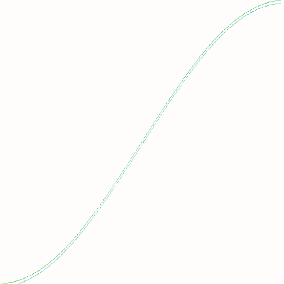
This graph shows cubic spline interpolation of cos(*x) on the interval [0,1] as well as the actual graph. They have been separated by 5 pixels to simplify viewing. The bottom graph is the actual function, the upper graph is the interpolated function. Note the similarity between thm.